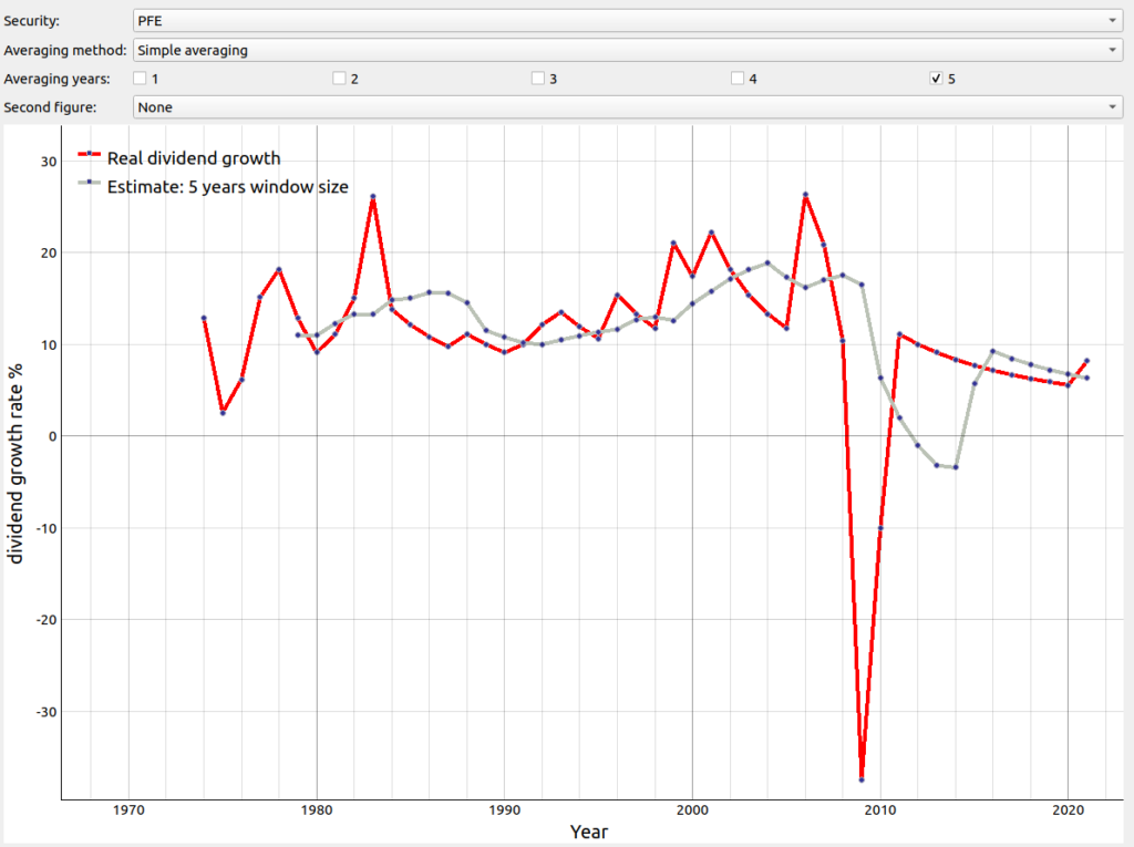
In the last blog entry Estimate dividend growth rate in the future part I different averaging technics were showed to estimate the next year’s dividend growth rate. In the figure below you can see again the rolling estimates for the dividend growth based on simple averaging (grey line) vs the real measured dividend growth rate (red line). As you can see there were quite some periods for which the estimated average was quite off. The interesting question would be: Can we quantify this deviation and then compare the different averaging techniques in order to make an informed decision on which one we should employ next?
The root-mean-square deviation
A good measure to gauche how well an estimation tracked the real values is the root-mean-square deviation. It is the square root of the sum of squared errors dividend by the number of samples:
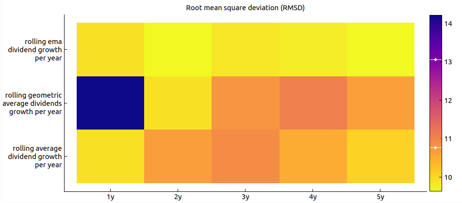
Figure 3 below illustrates the RMSDs for all potential filter technique combination with a color map for the security of PFE (Pfizer). As can be see for this security the filtering technique of rolling ema dividend with a window size of 5 years produced the smallest RMSD i.e. performed the best.
Just looking at the data of one security like in figure 3 might be not enough to decide which averaging technique to apply. Hence, the question arises whether there is a averaging method that is preferred independent of the securities in the portfolio. To evaluate this, we compared each strategy over a large set of stocks.
The best averaging method over several portfolios
In the last blog entry Estimate dividend growth rate in the future part I we have introduced the following three different averaging techniques to estimate next year’s dividend growth rate:
- Simple averaging last years’ growth rate
- Geometric averaging last years’ growth rate
- Exponential weighted average (EMA)
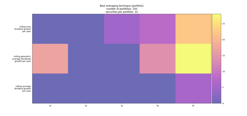
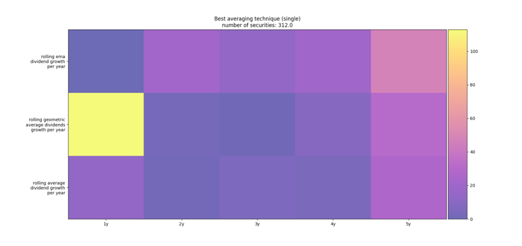
Furthermore, we have employed 5 different rolling window sizes in years for the averaging as also shown Github in the portfolio_tracker. To evaluate which combination of rolling window sizes is the best, we have constructed randomly 100 different portfolios with each portfolio containing 10 securities. The 10 securities of each portfolio were randomly selected from the all the stocks that are contained in the S&P 500 . The quant section on Github shows how to download all the ticker for the S&P 500 from Wikipedia. For every portfolio the average root-mean-square deviation per portfolio per strategy and per rolling window size was computed. Then we counted over all the portfolios the best averaging strategy. In figure 4 we have visualized the count array of the best strategy counted over all sample portfolios. As you can see there are two local maxima. On the one hand, it seems as the averaging technique of rolling geometric average as well as exponential moving average (top two rows) over a window size of 5 years performed very good. On the other hand, it seems as the averaging technique of rolling geometric averaging over only 1 year performed also very good. Please note, the latter averaging technique over the window size of last year is actually tantamount to saying that there is no change from last year’s dividend i.e. the growth rate is assumed to be 0%. These two results appear somewhat contradicting. We are going to analyze on why we observe this behavior. As you might notice the count array in figure 4 is weighted per portfolio and not per single stock. We did this because we believe ideally one would only need to employ one averaging technique over the whole portfolio and not per stock. However, it is possible that one “bad” sample in the portfolio could then skew the result of best averaging technique in an unfortunate way. Thus, we did the whole counting over the best averaging technique also per stock in all the 100 portfolios. This is shown in figure 5. As you can see the maximum lies now clearly on the filtering with rolling geometric averaging over only 1 year while there are still some securities for which the ema filtering over 5 years window size performed best. The reason for this discrepancy is that taking the last year’s estimate leads in average over a whole portfolio to a high root mean square error. The question to be answered is why did the technique of taking last year’s estimate perform so well for some stocks.
Why taking last year’s estimates works so well?
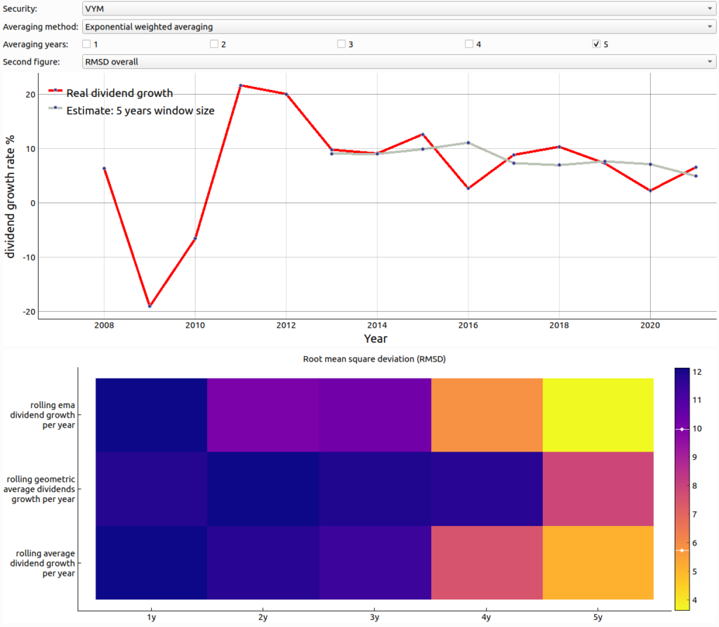
The averaging strategy rolling geometric average with a window size of one year which corresponds to taking last year’s estimate i.e. assumes 0% growth works extremely well as shown in the figures above for quite some stocks. To understand on why this is the case it is very instructive to compare the securities for which the last year’s estimate was best vs. securities for which the rolling ema over a window size of 5 year was best to estimate next year’s dividend growth. Let’s first consider and example for which the ema filtering works best. In the upper plot of the figure below you can see the real dividend growth (red line) vs the ema estimate (grey line) with a rolling window size of 5 years for the security VYM. As you can see the gray line tracks the red line quite close. Unsurprisingly, the root mean square deviation (RMSD) is only around 4% with this security and also best for this security as the lower plot of the visualization of the RMSDs for all potential estimation techniques nicely shows.
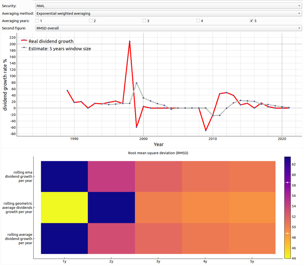
Now, let’s consider the same plots for security NWL in the figure below. As you can see in the upper plot there are several peaks in the dividend growth graph (red line) that are badly tracked by the estimate (grey line). What makes it worse is that there is some kind of zigzagging motion of the real dividend growth. This makes the estimate deviate not only while the peak occurs but also in the ensuing year. This behavior is responsible that assuming 0% growth in the ensuing year is superior for those stocks as visualized in the lower plot with the RMSD values for all potential filter techniques. As can be seen the RMSDs are very high for all filtering techniques in this scenario. Nevertheless assuming 0% growth trumps the others.
Conclusion
By comparing the different filter techniques and different window sizes by using the RMSD over different portfolios we could find the two best averaging techniques namely either rolling ema dividend growth per year with a window size of five years and rolling geometric average dividends growth per year with a window size of 1 i.e. assuming zero growth. We could show that assuming zero growth works best if there are a lot of fluctuation in the dividend growth rate. The question arises whether instead of just using one of two filtering techniques it wouldn’t be better to use a combined adaptive approach. This topic is planned to be analyzed in the next blog entry.