At the beginning of the year when I started to review my personal financial budget for 2022, I asked myself how the income that stems from dividends is going to develop in the new year. Clearly, I could model the additional dividends that I can collect from the additional investments I am going to make in the next year. However, this model requires to know how big the dividend per security is going to be. Obviously, one simple model would just assume that the dividend paid next year is the same as it was last year.

Why it is hard to estimate the dividend growth rate
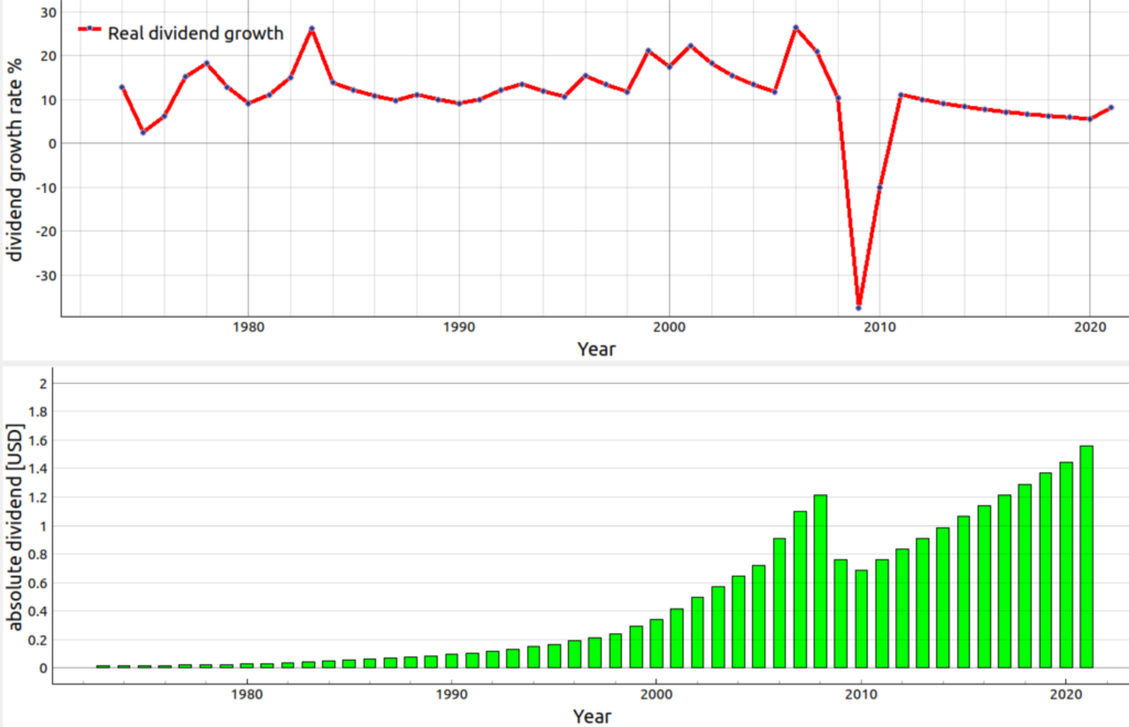
Ideally, the dividend growth rate would be constant. Since the dividend correlates strongly with a business’ earnings, the assumption cannot be made that the dividend or the growth rate remain constant indefinitely. Quite the opposite must be assumed over a long time horizon. As an example in the below plot you can see the dividend growth for the Pfizer share without any filtering in the upper plot. As you can see in the year 2009, there was a sharp drop into negative territory in the grow rate. This is a print screen from the finspresso portfolio tracker GUI that resides in the repository on Github. The reason for this drop was that the dividend was decreased from about 1.21 USD in the year 2008 to around 0.759 USD in the year 2009 due to the impact of the Great Recession. This illustrates that a forecast for dividend growth of a certain security based on a given dividend history might be wrong. Nevertheless, if one wants to forecast the next years income based on dividends it is important to at least model the dividend growth in some way. The next sections try to look into different approaches.
Taking last year’s growth rate
One approach would be to just to take the last years dividend growth rate as a estimate for next year’s dividend. I.e. the next year’s estimate of the dividend growth rate is the following:
One interesting aspect to consider here is how much the dividend growth rate changed from year to year. For the example of Pfizer you can see the distribution of the change in dividend growth in the figure below. As can be seen in the most cases the change in dividend growth year-over-year is in a range of +/-5% for this security.

Figure 2: Histogram showing the distribution of the change in dividend growth year-over-year for the security Pfizer.
Simple averaging last years’ growth rate
Another method would be to take the last years’ average of dividend growth rate:
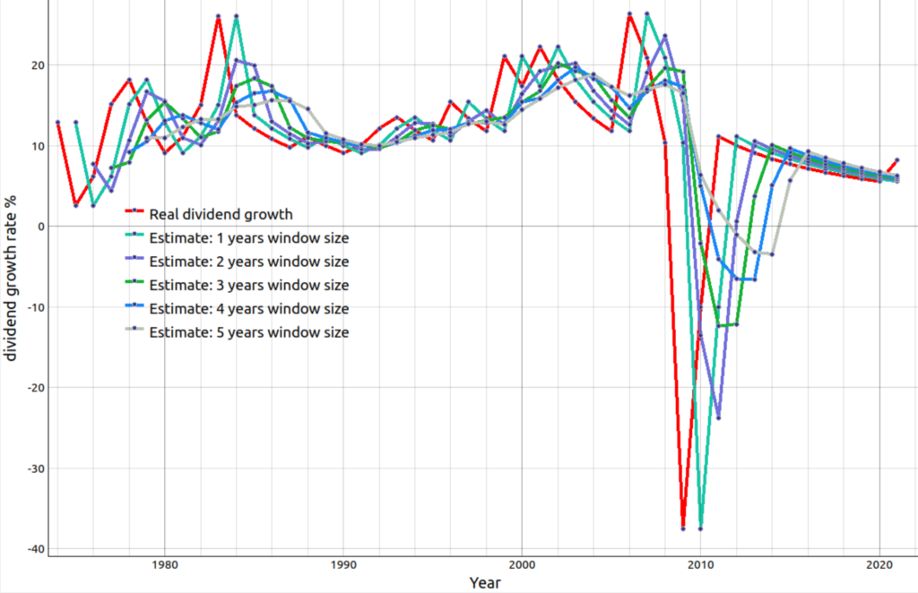
Looking at the formula above it is obvious that the averaged value predicates on the selected number of years. In Figure 3 below you can see the averaged dividend growth for the security Pfizer for different number of averaging years. There are 5 graphs for the rolling estimates. Every dividend estimation graph has a different rolling average window size. The longest widow is 5 years and the shortest 1 year. As can be seen the growth rate is most smooth if the years to average is the highest i.e. in this example 5. On the other hand, you can also see that in this case the estimate are sluggish by seeing that the rolling estimates take much longer to react to the drop in paid dividend in 2009.
Geometric averaging last years’ growth rate
A second method is to use the geometric mean to estimate the next years dividend growth rate. The geometric mean computes the annualized growth rate by considering the first and the last paid dividend over the considered time period as shown in this formula:
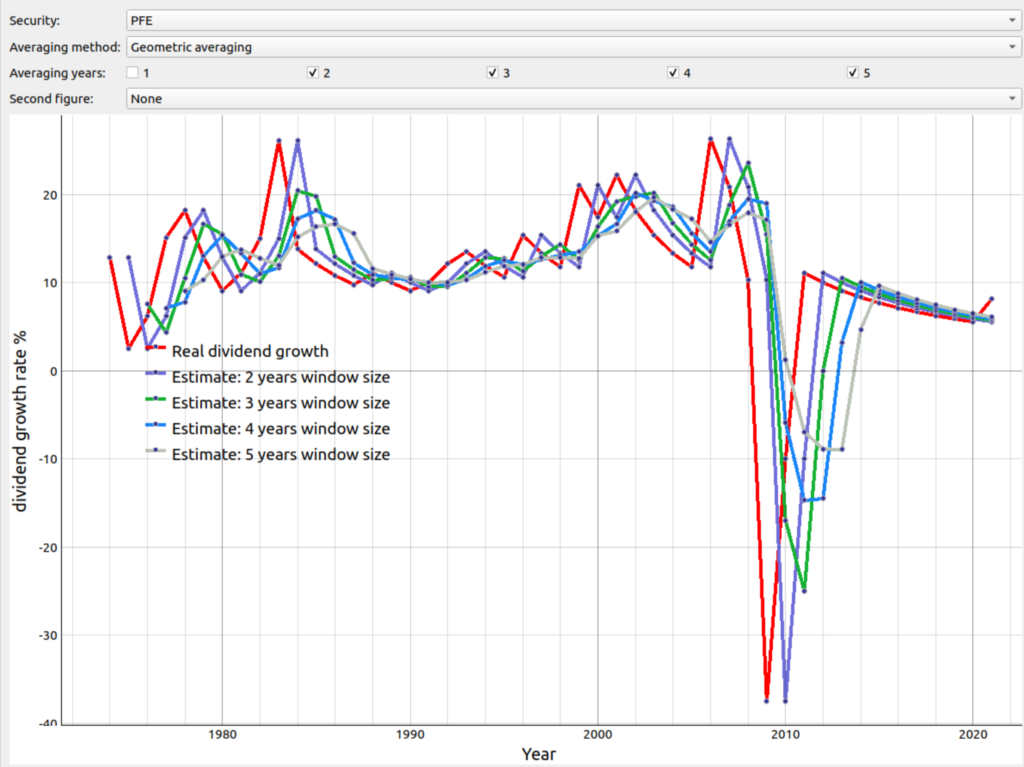
In the figure below you can see the graphs that show the geometric averaging of the dividend growth rate for the example of the company Pfizer with different rolling window sizes. Comparing this figure with figure 3 from above, you can see that when the window size i.e. number of years considered for the averaging process is high e.g. 5 the geometric averaging reacts much more than the simple averaging. This is visible around the year 2009. In the case of the simple averaging the gray line which symbolizes the rolling estimate for the next year for which the window size was 4 years estimated the dividend growth to be slightly above 5% for the year 2010. In reality the real growth in the year 2010 was -10% after it nosedived to below -37% in year 2009. Clearly taking the 6% as an estimate would have been off. On the hand other looking at the blue line in figure 4, we see that the estimate for the dividend growth for the year 2010 would have been -6% which is quite close to the -10%.
Exponential weighted average (EMA)
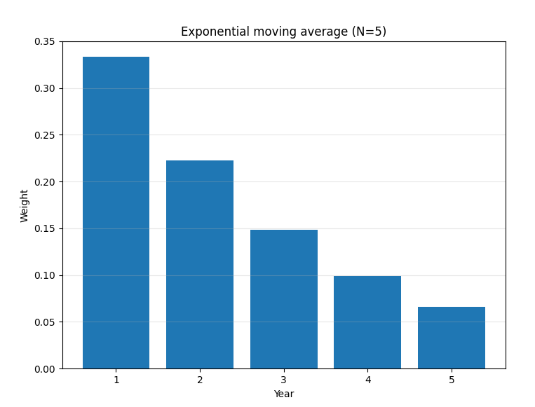
The potential downside of using a simple moving average filter as described above is that it gives each recorded dividend growth value in the past the same weight in the averaging. This makes the averaging more sluggish as shown for 5 years window size in figure 3. One potential way of mitigating this issue is to employ an exponential weighted average filter. The basic idea is to given more current measurements more weights than the older ones.
As an example consider the case where our averaging takes into account 5 measurements i.e. 5 years. In this scenario the different weighting factors in the averaging of the 5 elements are shown in figure 5:
In the figure below you can see the real dividend growth rate (red line) the rolling estimate with exponentially filtering with a window size of 5 years (gray) for the dividend growth of the company Pfizer. We see that that the exponentially averaged version over five years reacts much stepper than the geometric one did when averaging over the same time period as visible figure 4 respectively the simple averaging did as seen in figure 3.
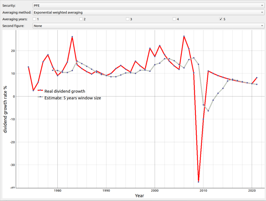
Figure 6: Dividend growth with exponential weighted averaging for window size of 5 years vs unfiltered.
Play around with tool on Github
This blog entry showed three different approaches how to estimate the dividend growth rate. While all seem to have their advantages and drawbacks it is not yet clear which performed the best. The goal of the next blog entry is to shed more light into this issue. If you want to see how the dividend growth rate looks with this GUI for other stocks, please visit the portfolio tracker on Github and follow the instruction in the the README. The financial data in the tool is downloaded from Yahoo Finance via the API Python wrapper yfinance. Please note, the given scripts are merely educational nature and should only used for personal usage according to the Yahoo terms of use (here, here and here).